How to model the Bernoulli distribution in Python
Bernoulli distribution is a particular case of the discrete probability distribution function (PDF) in which the number of observations is one, due to the conduction of a single experiment.
Bernoulli’s trial has two possible outcomes: success or failure, 1 or 0, yes or no, etc.
Formula
If p is the probability of an event having this distribution, and x is a random variable, then the probability mass function (PMF) of the Bernoulli distribution is as follows:
Here, x is either 0 or 1, and the value of p ranges from 0 to 1.
The mean of Bernoulli’s distribution is equal to p, while its variance is p(1-p).
Implementation in Python
SciPy is a built-in module of Python used for mathematical and scientific computations. The scipy.stats package is a sub-package that contains multiple probability distributions, frequency and summary statistics, masked statistics, correlation functions, statistical tests, and other features.
We use the scipy.stats package to import bernoulli in Python.
Syntax
from scipy.stats import bernoulli
Code
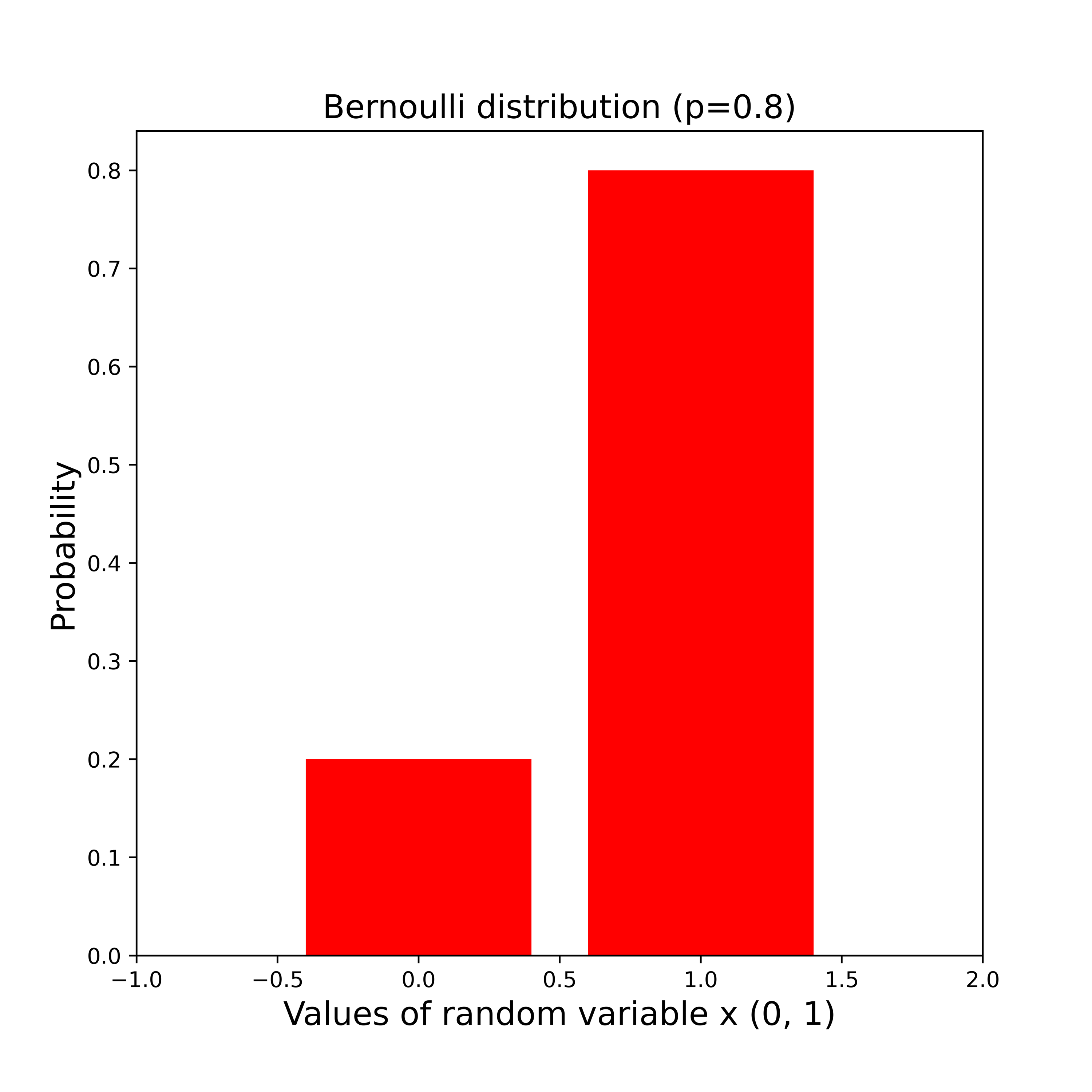
The Python code for the bar plot that uses the probability mass function to represent the Bernoulli distribution is given below.
This is a case of the Bernoulli distribution with p = 0.8. The outcome of the experiment can take the values of 0 and 1. The Bernoulli random variable’s values can be either 0 or 1.
We use the PMF function to calculate the probability of various random variable values.
# Import the required librariesfrom scipy.stats import bernoulliimport matplotlib.pyplot as plt# Instance of Bernoulli distribution with parameter p = 0.8bd=bernoulli(0.8)# Outcome of random variable either 0 or 1x=[0,1]# For the visualization of the bar plot of Bernoulli's distributionplt.figure(figsize=(10,10))plt.xlim(-2, 2)plt.bar(x, bd.pmf(x), color='blue')# For labelling of Bar plotplt.title('Bernoulli distribution (p=0.8)', fontsize='20')plt.xlabel('Values of random variable x (0, 1)', fontsize='20')plt.ylabel('Probability', fontsize='20')plt.show()
Explanation
- Lines 2–3: We import the required libraries.
- Line 6: We make an instance of Bernoulli’s distribution with the parameter
p=0.8. - Line 9: The experiment’s result could be
0or1, so we place it inx. - Lines 12–14: We use these commands to make a bar plot of the PDF of Bernoulli’s distribution.
- Lines 17–19: We label and title the bar plot.
Free Resources
