Random forest in Python
Random forest is an extension of the decision tree algorithm that builds multiple decision trees and combines their predictions to make more accurate and robust predictions. It creates a collection of decision trees, each trained on a random subset of data and features. This randomness helps to reduce overfitting and improve generalization.
Implementation
The following steps demonstrate the process of training and visualizing a random forest model using the provided dataset.
Step 1 - Importing the libraries
In the first step, we import the necessary libraries.
import numpy as npimport matplotlib.pyplot as pltimport pandas as pd
Step 2 - Importing the dataset
After importing libraries, we load the dataset from CSV file.
items = pd.read_csv('Data.csv')label1 = items.iloc[:, [2, 3]].valueslabel2 = items.iloc[:, 4].values
Here, we use iloc() function in Python to assign the variables label1 and label2 the values of the feature variable and the values of the target variable respectively from the dataset.
Step 3 - Splitting the dataset into training and test set
In this step, we split the data into training and test sets using the train_test_split function. The test set is set to be 25% of the entire dataset and random_state is used to ensure
from sklearn.model_selection import train_test_splitlabel1_train, label1_test, label2_train, label2_test = train_test_split(label1, label2, test_size = 0.25, random_state = 0)
Step 4 - Feature scaling
In this step, we scale the input features label1_train and label1_test to normalize the data.
from sklearn.preprocessing import StandardScalerscaling = StandardScaler()label1_train = scaling.fit_transform(label1_train)label1_test = scaling.transform(label1_test)
Step 5 - Fitting the model to the training dataset
Here, we fit the random forest model on the training dataset.
from sklearn.ensemble import RandomForestClassifiermodel = RandomForestClassifier(n_estimators=10, criterion='gini', random_state=0)model.fit(label1_train, label2_train)
Step 6 - Predicting the test set results
Here, we predict the target variable label2 for the label1_test.
prediction = model.predict(label1_test)from sklearn.metrics import confusion_matrixmatrix = confusion_matrix(label2_test, prediction)
We also make a confusion matrix to get the number of incorrect predictions.
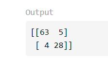
As we can see, here we have incorrect predictions in total.
Step 7 - The visualization of training set results
Then we create a scatter plot to visualize the decision boundaries of the trained random forest classifier on the training set.
from matplotlib.colors import ListedColormapseq1, seq2 = label1_train, label2_traingrid1, grid2 = np.meshgrid(np.arange(start = seq1[:, 0].min() - 1, stop = seq1[:, 0].max() + 1, step = 0.01),np.arange(start = seq1[:, 1].min() - 1, stop = seq1[:, 1].max() + 1, step = 0.01))plt.contourf(grid1, grid2, model.predict(np.array([grid1.ravel(), grid2.ravel()]).T).reshape(grid1.shape),alpha = 0.75, cmap = ListedColormap(('lightblue', 'peachpuff')))plt.xlim(grid1.min(), grid1.max())plt.ylim(grid2.min(), grid2.max())for key, value in enumerate(np.unique(seq2)):plt.scatter(seq1[seq2 == value, 0], seq1[seq2 == value, 1],c = ListedColormap(('mediumturquoise', 'lightsalmon'))(key), label = value)plt.title('Training set of random forest')plt.xlabel('Age')plt.ylabel('Estimated salary')plt.legend()plt.savefig('output/1_training.png')
Here we saved the visualization generated by the code as an image file named 1_training.png in the specified folder output using plt.savefig.
Step 8 - The visualization of test set results
Similarly, we create a scatter plot to visualize the decision boundaries of the trained random forest classifier on the test set.
from matplotlib.colors import ListedColormapseq1, seq2 = label1_test, label2_testgrid1, grid2 = np.meshgrid(np.arange(start = seq1[:, 0].min() - 1, stop = seq1[:, 0].max() + 1, step = 0.01),np.arange(start = seq1[:, 1].min() - 1, stop = seq1[:, 1].max() + 1, step = 0.01))plt.contourf(grid1, grid2, model.predict(np.array([grid1.ravel(), grid2.ravel()]).T).reshape(grid1.shape),alpha = 0.75, cmap = ListedColormap(('lightblue', 'peachpuff')))plt.xlim(grid1.min(), grid1.max())plt.ylim(grid2.min(), grid2.max())for key, value in enumerate(np.unique(seq2)):plt.scatter(seq1[seq2 == value, 0], seq1[seq2 == value, 1],c = ListedColormap(('mediumturquoise', 'lightsalmon'))(key), label = value)plt.title('Test set of random forest')plt.xlabel('Age')plt.ylabel('Estimated salary')plt.legend()plt.savefig('output/2_testing.png')
Here we saved the visualization generated by the code as an image file named 2_testing.png in the specified folder output using plt.savefig.
Code
import numpy as npimport matplotlib.pyplot as pltimport pandas as pditems = pd.read_csv('Data.csv')label1 = items.iloc[:, [2, 3]].valueslabel2 = items.iloc[:, 4].valuesfrom sklearn.model_selection import train_test_splitlabel1_train, label1_test, label2_train, label2_test = train_test_split(label1, label2, test_size = 0.25, random_state = 0)from sklearn.preprocessing import StandardScalerscaling = StandardScaler()label1_train = scaling.fit_transform(label1_train)label1_test = scaling.transform(label1_test)from sklearn.ensemble import RandomForestClassifiermodel = RandomForestClassifier(n_estimators=10, criterion='gini', random_state=0)model.fit(label1_train, label2_train)prediction = model.predict(label1_test)from sklearn.metrics import confusion_matrixmatrix = confusion_matrix(label2_test, prediction)print(matrix)from matplotlib.colors import ListedColormapseq1, seq2 = label1_train, label2_traingrid1, grid2 = np.meshgrid(np.arange(start = seq1[:, 0].min() - 1, stop = seq1[:, 0].max() + 1, step = 0.01),np.arange(start = seq1[:, 1].min() - 1, stop = seq1[:, 1].max() + 1, step = 0.01))plt.contourf(grid1, grid2, model.predict(np.array([grid1.ravel(), grid2.ravel()]).T).reshape(grid1.shape),alpha = 0.75, cmap = ListedColormap(('lightblue', 'peachpuff')))plt.xlim(grid1.min(), grid1.max())plt.ylim(grid2.min(), grid2.max())for key, value in enumerate(np.unique(seq2)):plt.scatter(seq1[seq2 == value, 0], seq1[seq2 == value, 1],c = ListedColormap(('mediumturquoise', 'lightsalmon'))(key), label = value)plt.title('Training set of random forest')plt.xlabel('Age')plt.ylabel('Estimated salary')plt.legend()plt.savefig('output/1_training.png')plt.show()from matplotlib.colors import ListedColormapseq1, seq2 = label1_test, label2_testgrid1, grid2 = np.meshgrid(np.arange(start = seq1[:, 0].min() - 1, stop = seq1[:, 0].max() + 1, step = 0.01),np.arange(start = seq1[:, 1].min() - 1, stop = seq1[:, 1].max() + 1, step = 0.01))plt.contourf(grid1, grid2, model.predict(np.array([grid1.ravel(), grid2.ravel()]).T).reshape(grid1.shape),alpha = 0.75, cmap = ListedColormap(('lightblue', 'peachpuff')))plt.xlim(grid1.min(), grid1.max())plt.ylim(grid2.min(), grid2.max())for key, value in enumerate(np.unique(seq2)):plt.scatter(seq1[seq2 == value, 0], seq1[seq2 == value, 1],c = ListedColormap(('mediumturquoise', 'lightsalmon'))(key), label = value)plt.title('Test set of random forest')plt.xlabel('Age')plt.ylabel('Estimated salary')plt.legend()plt.savefig('output/2_testing.png')plt.show()
Conclusion
In conclusion, the random forest algorithm effectively handles complex datasets and makes accurate predictions. When using random forest, it's essential to experiment with different hyperparameters and criteria to achieve the best performance for a specific task.
Free Resources