The basics of Matrix calculus for Deep Learning

Credits: Based on the paper, “The Matrix Calculus You Need For Deep Learning” by Terence Parr and Jeremy Howard. Thanks for this paper.

The paper mentioned above is beginner-friendly, but I wanted to write this shot to note points that would make it much easier to understand the paper. When I learn topics that are slightly difficult, I find it helps to explain it to a beginner, so this shot is for a beginner.

Deep Learning is all about linear algebra and calculus. If you try to read any deep learning paper, matrix calculus will be needed to understand the concept.

I have written my understanding of the paper mentioned above in the form of three shots. This is part 1, check out parts 2, and 3.

Deep learning is basically the use of neurons with many layers, but what does each neuron do?

Introduction

Each neuron applies a function on an input and gives an output. The activation of a single computation unit in a neural network is typically calculated using the dot product of an edge weight vector (w) with an input vector (x) plus a scalar bias (threshold):

z(x) = w · x + b

Where the letters written in bold are vectors.

Function z(x) is called the unit’s affine function and is followed by a rectified linear unit that clips negative values to zero: max(0, z(x)). This computation takes place in neurons. Neural networks consist of many of these units organized into multiple collections of neurons called layers. The activation of one layer’s units is the input to the next layer’s units. Math becomes simple when inputs, weights, and functions are treated as vectors, and the flow of values is treated as matrix operations.

The most important math used here is differentiationcalculating the rate of change and optimizing the loss function to decrease error. Training phase is all about choosing weights (w) and bias (b) so that we get the desired output for all N inputs (x). To do that, we minimize a loss function. To minimize the loss, we use SGDStochastic gradient descent is an iterative method for optimizing an objective function with suitable smoothness properties.. Measuring how the output changes with respect to a change in weight is the same as calculating the (partial) derivative of the output w.r.t weight (w). All of these require the partial derivative (the gradient) of activation (x) with respect to the model parameters (w) and b. Our goal is to gradually tweak w and b so that the overall loss function keeps getting smaller across all x inputs.

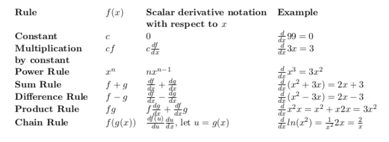
Scalar derivative rules

Below are the basic rules you will need to solve this problem:

Partial derivatives

Neural networks are functions of multiple parameters; let’s discuss that.

What is the derivative of xy(multiply x and y)?

Well, it depends on whether we are changing it with respect to x or y. We compute derivatives with respect to one variable at a time, which, in this case, gives two derivatives. We call these partial derivatives. δ is the symbol used instead of d to represent partial derivatives. The partial derivative, with respect to x, is just the usual scalar derivative that treats any other variable in the equation as a constant.

Matrix calculus

You can see how we would calculate the gradient of (x,y) below:

The gradient of f(x,y) is simply a vector of its partials. Gradient vectors organize all of the partial derivatives for a specific scalar function. If we have two functions, we can organize their gradients into a matrix by stacking the gradients. When we do so, we get the Jacobian matrix, where the gradients are rows.

To define the Jacobian matrix more generally, let’s combine multiple parameters into a single vector argument:

f (x, y, z) ⇒ f (x)

Let y = f (x) be a vector of (m) scalar-valued functions that each take a vector (x) of length n = |x|, and where |x| is the cardinality (count) of elements in x. Each f of i is a function within f that returns a scalar. For example, f (x, y) = 3x²y and g(x, y) = 2x + y⁸ from the last section as:

y₁ = f₁(x) = 3x²₁x₂

y₂ = f₂(x) = 2x₁ + x⁸₂

The Jacobian matrix is a collection of all m × n possible partial derivatives (m rows and n columns) that is the stack of m gradients with respect to x.

The Jacobian matrix of the identity function f(x) = x, with fi (x) = x i , has n functions and each function has n parameters that are held in a single vector (x). Therefore, since m = n, Jacobian is a square matrix.

Element-wise operations on vectors

Element wise operations are important to know in deep learning. By Element-wise binary operations, we mean the application of an operator to the first item of each vector to get the first item of the output, then to the second items of the inputs for the second item of the output, and so on. We can generalize the element-wise binary operations with the notation:

y = f (w) O g(x) where m = n = |y| = |w| = |x|

Derivatives involving scalar expansion

When we multiply or add scalars to vectors, we’re implicitly expanding the scalar to a vector and then performing an element-wise binary operation. For example:

(The notation -> 1 represents a vector of 1’s appropriate length.) z is any scalar that doesn’t depend on x, which is useful because then ∂z/∂x= 0 for any x i. This will simplify our partial derivative computations.

Vector sum reduction

Summing up the elements of a vector is an important operation in deep learning (similar to the network loss function).

Let y = sum(f (x))

Notice how we were careful here to leave the parameter as a vector (x) because each function f i could use all the values in the vector, not just x i . The sum is over the results of the function and not the parameter.

In the gradient of the simple y = sum(x)= [1,1 …1], because ∂x i/ ∂x j = 0 for j != i, transpose since we have assumed the default to be vertical vectors. It is very important to keep the shape of all of your vectors and matrices in order; otherwise, it’s impossible to compute the derivatives of complex functions.

This is part 1. In part 2, I will explain the chain rule.