The Principles of the Convolution

Learn about the convolution operation and how it is used in deep learning.

We'll cover the following

Why convolution?

The fully connected layer that we saw doesn’t respect the spatial structure of the input. If, for example, the input is an image, the NN will destruct the 2D structure into a 1-dimensional vector. To address the issue, we have designed Convolutional Neural Networks (CNNs). They work exceptionally well for computer vision applications.

Why do we use them when we process images? Because we know a priori that nearby pixels share similar characteristics and we want to take that into account by design. That assumption is called the inductive bias.

Convolutional layers exploit the local structure of the data.

Representation of a Convolutional Neural Network

But how is it possible to focus on the local structure instead of fully connected layers that take linear combinations of the input?

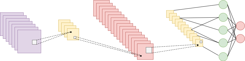
The answer is quite simple. We restrict the convolutional layer to operate on a local window called kernel. Then, we slide this window throughout the input image.

Convolution

The basic operation of CNNs is the convolution. Mathematically, a convolution between two 2-dimensional functions is defined as:

(fg)(i,j)=abf(a,b)g(ia,jb).(f*g)(i,j) = \sum_{a} \sum_{b} f(a,b)g(i-a,j-b).

Even though one signal is inverted in maths before the sliding, in deep learning, this is ignored. The reason is that our weights inside the kernel will be trainable.

Convolution between two signals

Visually, we can represent a 2x2 kernel operating in a 4x4 image as follows:

The convolution operation

Try to slide the kernel in the image. Note that each operation between the kernel and the image will be a dot product, which produces a scalar (shown in blue in the output).

The output is called a feature map.

We can see that given a matrix (our input) and a smaller weight matrix (kernel), we can produce a single scalar number. This number is essentially the result of the dot product between a small chunk of our input with the kernel.

It is interesting to understand that this dot product is a measure of correlation (similarity). CNNs are great at learning the spatial correlations of neighboring pixels.

Below is an example of a 3x3 chunk of the image (called patch) with a 3x3 kernel:

fg=[abcdefghi][123456789]f*g = \begin{bmatrix}a & b & c \\ d & e & f \\g & h & i \end{bmatrix} * \begin{bmatrix} 1 & 2 & 3 \\4 & 5 & 6 \\7 & 8 & 9 \end{bmatrix}

fg=(a1)+(b2)+(c3)+(d4)+(e5)+(f6)+(g7)+(h8)+(i9)f*g = (a\cdot1) +(b\cdot2) +(c\cdot3) + (d\cdot4) + (e\cdot5) + (f\cdot6)+ (g\cdot7) + (h\cdot8) + (i\cdot9)

Again, it is simply a dot-product.

To recap: Given an input matrix N×NN \times N and a kernel p×pp \times p, where p<N:

  • We slide the filter across every possible position of the input matrix.
  • At each position, we perform a dot-product operation and calculate a scalar.
  • We gather all these scalar together to form the output, which is called the feature map.

So what did we achieve here?

We transformed a 2D matrix from the input space to the feature space but without losing the 2D form of the input. That way the network can capture context that only appears in parts of the image and would otherwise be lost by a fully connected layer.

Intuitively, CNNs are able to recognize patterns in images such as edges, corners, circles, etc. From another perspective, CNNs can be thought of as locally connected neural networks — as opposed to fully connected — because each pixel of the feature map is affected only by a local region of the input rather than the entire image.

Important notes

  • Convolution is still a linear operator.
  • The weights that are in the kernel are trainable and are shared through the input.
  • Each dot-product operation gives a notion of similarity.
  • Convolutional layers can be performed in any number of dimensions.
  • The axis that we slide the image on defines the dimension of a convolution. For images, it is a 2D convolution. But we can still apply convolutions in 1D sequences that have some kind of local structure.

If you understand the basics of convolution, you should be able to implement convolution from scratch in Python. It is just a few lines of code. In the exercise below, you have a simple function that receives a 2D image and a 2D kernel. The goal is to output the result of their convolution.

Your code will be tested in 4 different images. The kernel will always be of size (3, 3) and the images will be (8, 8), (12, 10), (10, 10), and (12, 8) respectively.

Get hands-on with 1200+ tech skills courses.