...
/Probability Distributions (Binomial and Bernoulli Distributions)
Probability Distributions (Binomial and Bernoulli Distributions)
Knowledge of Probability Distributions is essential in the Data Science field and it is the backbone for understanding many concepts. You'll learn about it in this lesson.
We'll cover the following...
What are probability distributions ?
Probability distribution is a summary of probabilities associated with all the possible outcomes of a random variable X. Probability Distributions have a particular shape that has properties like Mean(Expected Value), Variance, Skewness and Kurtosis.
Example
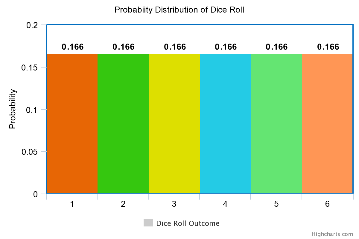
When we roll a fair dice, the probability of each outcome is equally likely, meaning . We can write it as seen below.
| Outcome of Rolling a Dice | Probability |
|---|---|
| 1 | 1/6 |
| 2 | 1/6 |
| 3 | 1/6 |
| 4 | 1/6 |
| 5 | 1/6 |
| 6 | 1/6 |
Probability Histogram
If we take the dice roll outcome on the x-axis and its probability on the y-axis, we get the below graph representation.
Types of random variables
Discrete random variables
Discrete random variables are the variables whose outcomes take on a discrete set of values. The function that calculates the probability of each outcome (Probability Distribution) of a Discrete Random Variable is called the Probability Mass Function.
Example
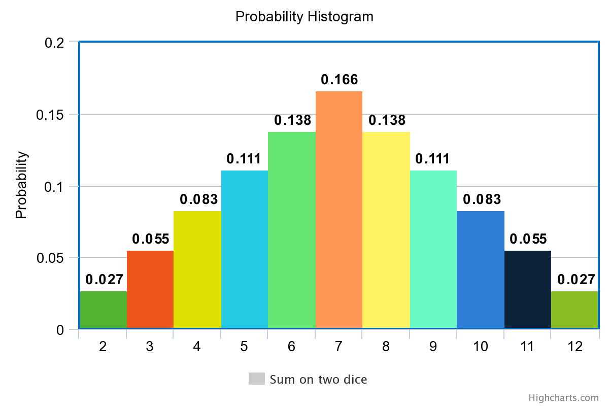
Let X be the random variable denoting the sum of two dice. When two dice are rolled, the possible outcomes on the face of the dices are (1,1), (1,2), (1,3), (1,4) , (1,5), (1,6), (2,1), (2,2) and so on. So the total outcomes are 36, among which the possible sum on two dices are listed below along with their probability.
| X (the sum of two dice) | Probability |
|---|---|
| 2 | 1/36 |
| 3 | 2/36 |
| 4 | 3/36 |
| 5 | 4/36 |
| 6 | 5/36 |
| 7 | 6/36 |
| 8 | 5/36 |
| 9 | 4/36 |
| 10 | 3/36 |
| 11 | 2/36 |
| 12 | 1/36 |
Probability Histogram
If we take the sum of the two dice on the x-axis and their probability on the y-axis, we get the below graph representation.
Continuous Random Variables
The variable whose outcomes can take on a real value. The Probability Density Function (PDF) defines the probability distribution of a Continuous Random Variable. Notice that for Discrete Random Variable it was called Probability Mass Function.
A continuous random variable has a probability of zero of assuming exactly any of its values. Consequently, its probability distribution cannot be given in tabular form.
The probability distribution of a Continuous Random Variable is shown by a density curve. The probability that X is between an interval of numbers is the area under the density curve between the interval endpoints. One of the most commonly used Continuous Probability Distribution is Gaussian or Normal Distribution.
Bernoulli Distribution
Bernoulli Distribution is a Discrete Probability Distribution. Bernoulli Distribution consists of only two outcomes: 1 (success) and 0 (failure). The probability of success is denoted by “p”, and the probability of failure is denoted by “q” or “1-p”.
The Probability Mass Function which calculates the probability of each outcome is given as
= = ...