Data Structures 101 in 2026: introducing graphs in JavaScript
Master graph data structures in JavaScript by learning graph representations, BFS, DFS, shortest path algorithms, spanning trees, and real-world applications. Build the algorithmic foundation needed for coding interviews and software engineering.
In computer programming, data structures are used to organize data and apply algorithms (or commands) to code. Having a good understanding of data structures is essential for coding beginners and senior devs alike. In fact, questions related to data structures are some of the most common for entry-level interviews.
Today we will be looking at the graph data structure, one of the most widely-used data structures with applications across computing, mathematics, and other related fields.
Master data structures for coding interviews with hands-on practice
Learn all about graphs by studying real-world coding interview challenges
What is a graph?#
When we talk about graphs, the first thing that likely comes to mind is the conventional graphs used to model data. In computer science, the term has a completely different meaning.
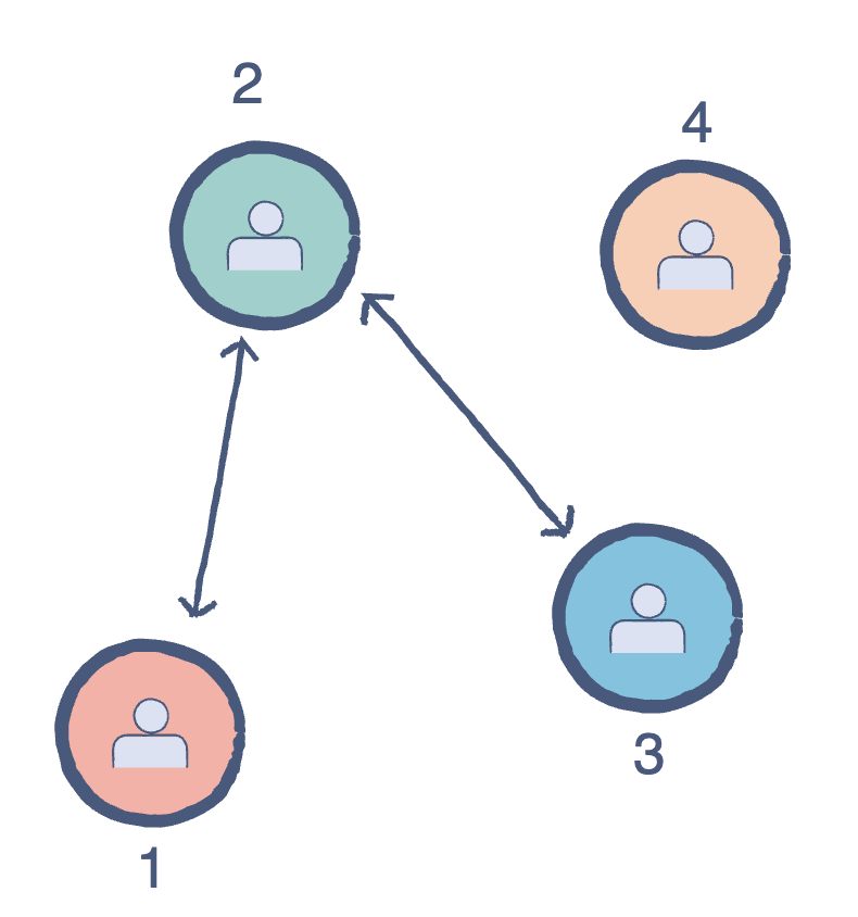
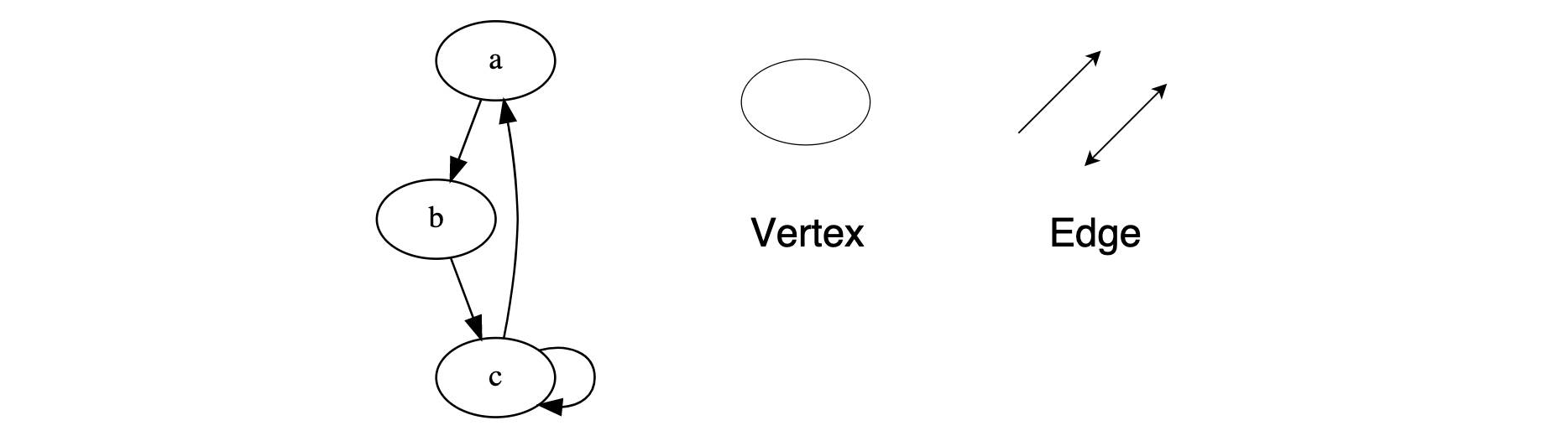
In programming, a graph is a common data structure that consists of a finite set of nodes (or vertices) and edges. The edges connect the vertices to form a network. An edge can be uni-directional or bi-directional. Edges are also known as arrows in a directed graph and may contain values that show the required cost to traverse from one vertex to another.
A vertex is similar to linked list nodes. A pair (x,y) is referred to as an edge. This communicates that the x vertex connects to the y vertex.
Graph terminology#
Let’s explore some common terminologies you’ll come across when working with graphs. To be successful with graphs, it’s important to understand the key terms to develop a grasp of how the different properties interact with each other relationally. Let’s take a look.
Degree of a vertex: The total number of edges connected to a vertex. There are two types of degrees:
-
In-Degree: The total number connected to a vertex.
-
Out-Degree: The total of outgoing edges connected to a vertex.
Adjacency: Two vertices are said to be adjacent if there is an edge connecting them directly.
Parallel Edges: Two undirected edges are parallel if they have the same end vertices. Two directed edges are parallel if they have the same origin and destination.
Self Loop: This occurs when an edge starts and ends on the same vertex.
Isolated vertex: A vertex with zero degree, meaning it is not an endpoint of an edge.
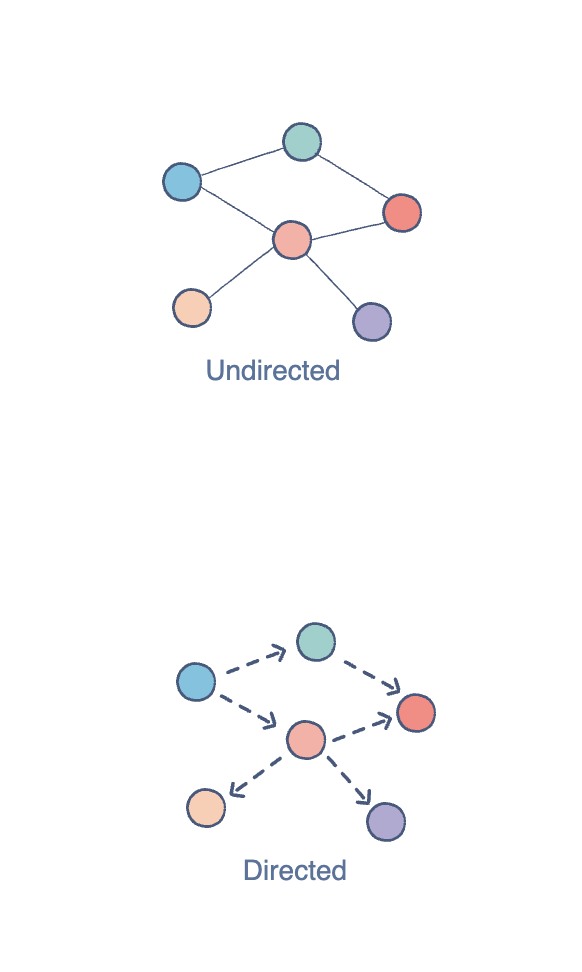
There are two common types of graphs. In an undirected graph, the edges are bi-directional by default; for example, with the pair (0,1), it means there exists an edge between vertex 0 and 1 without any specific direction. You can go from vertex 0 to 1, or vice versa.
Say we wanted to calculate the maximum possible edges for an undirected graph. The maximum possible edges of a graph with n vertices will be all possible pairs of vertices. There are possible pairs of vertices, according to Combinatorics. Solving by binomial coefficients gives us , so there are maximum possible edges in an undirected graph.
In a directed graph, the edges are unidirectional; for example, with the pair (0,1), it means there exists an edge from vertex 0 towards vertex 1, and the only way to traverse is to go from 0 to 1.
This changes to the number of edges that can exist in the graph. For a directed graph with vertices, the minimum number of edges that can connect a vertex with every other vertex is . So, if you have n vertices, then the possible edges is .
Types of graph representations#
We can represent a graph in different ways when trying to solve problems in our systems. In this section, we will take a look at the two most commonly used representations: Adjacency List and Adjacency Matrix.
Adjacency Matrix#
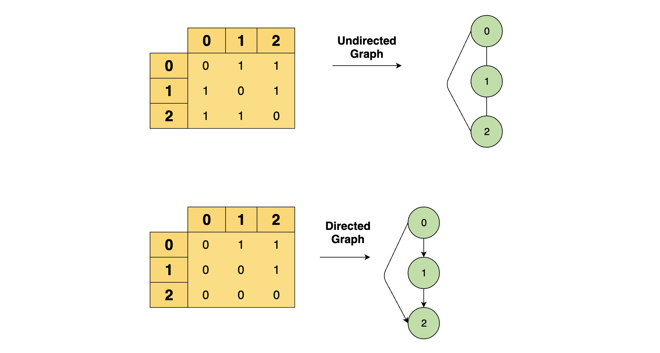
The adjacency matrix is a two-dimensional matrix where each cell can contain a 0 or a 1. The row and column headings represent the source and destination vertices respectively. If a cell contains 1, that means there’s an edge between the corresponding vertices. Edge operations are performed in constant time, as we only need to manipulate the value in the particular cell.
Master data structures for coding interviews.#
Learn data structures and algorithms in JavaScript without scrubbing through videos or documentation. Educative’s text-based courses are easy to skim and feature live coding environments, making learning quick and efficient.
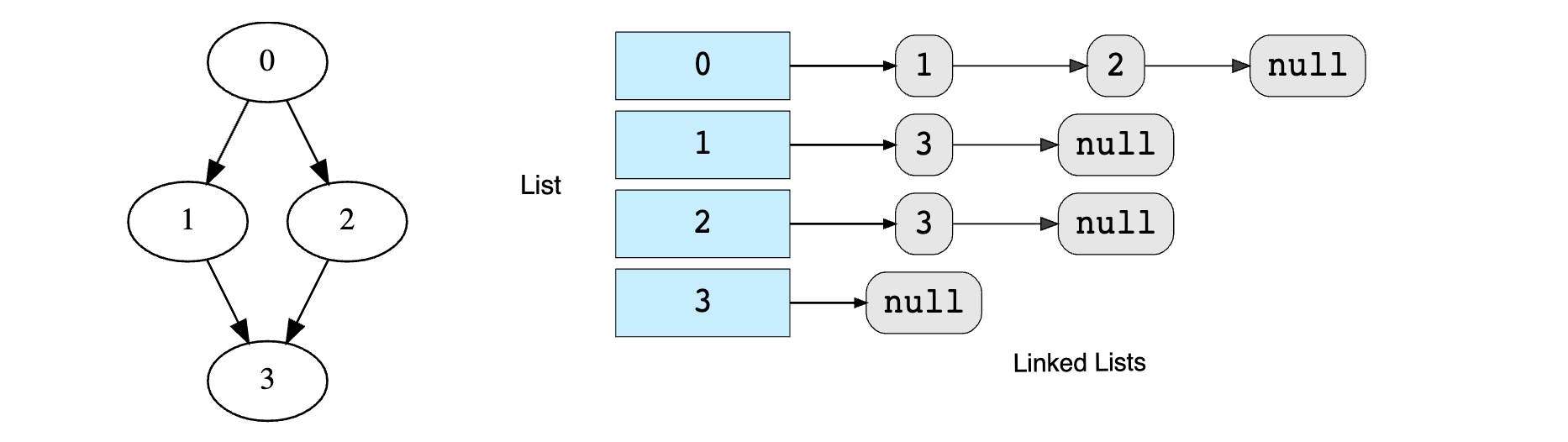
Adjacency List#
In an Adjacency List, an array of Linked Lists is used to store edges between two vertices. The size of the array is equal to the number of vertices. Each index in this array represents a specific vertex in the graph. If a new vertex is added to the graph, it is simply added to the array as well.
Adding an edge and a vertex to the Adjacency List is also a time-constant operation. Removing an edge takes time because–in the worst case–all the edges could be at a single vertex. Therefore, we would traverse all E edges to reach the last one. Removing a vertex takes time because we have to delete all its edges and then reindex the rest of the list one step back.
Use cases: Both representations are suitable for different situations. If your model frequently manipulates vertices, the adjacency list is a better choice. If you are dealing primarily with edges, the adjacency matrix is the more efficient approach.
How to implement a graph in JavaScript#
We’ve taken a look at graphs from a theoretical viewpoint. Let’s now try to implement a graph in code. After all, the best way to learn data structures is to use them with real data. The implementation below uses JavaScript and will be based on the Adjacency List representation.
As we know, the Graph class consists of two data members:
- The total number of vertices in the graph
- An array of linked lists to store adjacent vertices
Here, we’ve laid down the foundation of our Graph class. The variable vertices contains an integer specifying the total number of vertices. The second component is an array, which will act as our adjacency list. We simply have to run a loop and create a linked list for each vertex. Now, we’ll add two methods to make this class functional:
printGraph(): This prints the contents of the graphaddEdge(): This connects a source with a destination
addEdge (source, destination)#
Source and destination are already stored as index of our array. This function inserts a destination vertex into the adjacency linked list of the source vertex using the following line of code:
this.list[source].insertAtHead(destination)
We implementing a directed graph, so addEdge(0, 1) does not equal addEdge(1, 0).
printGraph()#
This function uses a nested loop to iterate through the adjacency list. Each linked list is being traversed.
What about an undirected graph?
So far, we have covered the implementation of a directed graph.
For an undirected graph, we we create an edge from the source to the destination and from the destination to the source. This makes it a bidirectional edge.
Graph traversal algorithms#
As we have previously mentioned, when we move through a graph, we are traversing the data. This refers to the process of visiting the vertices of a graph. Traversal processes are classified by the order that the vertices are visited. This is similar to tree traversal. Let’s get into the basic logic behind graph traversal and see how we can use algorithms to do it.
When traversing graphs, we use the concept of levels. Take a vertex as your starting point; this is the lowest level. The next level is all the adjacent vertices. A level higher would be the vertices adjacent to these nodes.
The two basic techniques for graph traversal are:
-
Breadth-First Search (BFS): The BFS algorithm grows breadth-wise. All the nodes at a certain level are traversed before moving on to the next level. This level-wise expansion ensures that for any starting vertex, you can reach all others one level at a time.
-
Depth-First Search (DFS): This algorithm is the opposite of BFS; it grows depth-wise. Starting from any node, we move to an adjacent node until we reach the farthest level. Then we move back to the starting point and pick another adjacent node. Once again, we probe to the farthest level and move back. This process continues until all nodes are visited.
When should you use BFS vs DFS?#
Understanding how BFS and DFS work is important, but knowing when to use each algorithm is often more valuable in practice. While both algorithms traverse a graph, they excel at solving different types of problems.
Breadth-First Search is typically the preferred choice when you need to find the shortest path in an unweighted graph or explore nodes level by level. Because BFS visits all vertices at the current depth before moving deeper into the graph, it naturally discovers the shortest route between two nodes when all edges have equal weight. This makes it useful for applications such as social network connections, network routing, and shortest-path interview problems.
Depth-First Search is often a better fit when exploring an entire graph structure, detecting cycles, performing topological sorting, or solving backtracking problems. Since DFS follows a path as deeply as possible before returning, it is particularly effective for tasks that require exhaustive exploration of relationships and dependencies.
As you practice graph problems, one useful rule of thumb is to think of BFS as the algorithm for finding the nearest solution and DFS as the algorithm for thoroughly exploring possibilities.
Shortest Paths and Weighted Graphs#
Graphs with weights (costs) unlock a rich set of problems — from route planning and network latency to optimizing supply chains.
Solving these efficiently requires specialized algorithms for weighted traversal.
Dijkstra’s Algorithm (for non-negative weights)#
Use a priority queue (min-heap) to compute shortest paths from a source node:
function dijkstra(graph, start) {const dist = {};const pq = new MinPriorityQueue();for (let v in graph.adjList) dist[v] = Infinity;dist[start] = 0;pq.enqueue(start, 0);while (!pq.isEmpty()) {const { element: u } = pq.dequeue();for (let [v, weight] of graph.adjList[u]) {const alt = dist[u] + weight;if (alt < dist[v]) {dist[v] = alt;pq.enqueue(v, alt);}}}return dist;}
When weights can be negative#
If edge weights may be negative, use:
Bellman–Ford for single-source shortest paths
Johnson’s algorithm for all-pairs shortest paths
Common applications#
Finding the fastest route in a navigation system
Computing shortest paths in weighted social or network graphs
Minimizing costs in logistics, pipelines, or data routing
Complexity#
With an adjacency list and a min-heap, Dijkstra’s algorithm runs in
O((V + E) log V) — efficient enough for large, sparse graphs.
Understanding these patterns shows you can extend recursion and traversal ideas into weighted optimization problems, a hallmark of strong algorithmic fluency.
Spanning trees, connectivity, and graph decomposition#
Minimum Spanning Tree (MST)#
For undirected weighted graphs, MST finds a subset of edges that connects all vertices with minimal total weight:
Kruskal’s algorithm: sort edges, union-find for connectivity.
Prim’s algorithm: grow from a seed vertex using a priority queue.
MST applications:
Designing least-cost network infrastructure (roads, fiber).
Clustering approaches: MST can be the backbone of hierarchical clustering.
Strongly Connected Components & Topological Sort#
For directed graphs:
Kosaraju’s or Tarjan’s algorithm finds strongly connected components (SCCs).
Topological sort orders vertices linearly in a Directed Acyclic Graph (DAG). Use DFS post-order or Kahn’s algorithm.
Use cases:
Scheduling jobs with dependencies (build systems, course prerequisites).
Condensing a complex directed graph into SCCs for high-level abstractions.
Advanced Traversal and Cycle Detection#
Depth-First Search (DFS) isn’t just for visiting nodes — it’s a foundation for solving many graph structure problems.
What DFS can do#
Detect cycles
In directed graphs, maintain a recursion stack to spot back edges.
In undirected graphs, track parent pointers to avoid false positives.
Backtrack paths or find all paths
Keep a current path list and backtrack after exploring each neighbor.
Reconstruct specific paths
During BFS or DFS, store parent pointers so you can rebuild the route later.
Iterative DFS with a stack
Use this version to avoid recursion depth limits, especially in JavaScript.
Example: Cycle detection in a directed graph#
function hasCycle(graph) {const visited = {}, recStack = {};function dfs(v) {visited[v] = true;recStack[v] = true;for (let [u, w] of graph.adjList[v]) {if (!visited[u]) {if (dfs(u)) return true;} else if (recStack[u]) {return true;}}recStack[v] = false;return false;}for (let v in graph.adjList) {if (!visited[v] && dfs(v)) return true;}return false;}
By mastering DFS for cycle detection, path reconstruction, and iterative exploration, you can tackle a wide range of graph interview questions efficiently — from dependency resolution to pathfinding.
Real-world uses of graphs#
Graphs are used to solve real-life problems that involve representation of the problem space as a network. Any network related application (paths, finding relationships, routing, etc.) apply the concept of graphs. Therefore, the graph data structure plays a fundamental role in several applications:
- GPS
- Neural networks
- Peer to peer networks
- Search engine crawlers
- Garbage collection
- Social networking websites
- and more
For example, a single user on Facebook can be represented as a node (vertex), while their connection with others can be represented as an edge between nodes, and each node can be a structure that contains information like the user’s id, name, location, etc.
Graphs are being used to improve the efficiency of the applications we use daily. These are a fundamental part of our day-to-day lives.
-
Facebook Graph API, for example, uses the concept of graphs, where users are considered to be the vertices and an edge runs between friends and other entities such as comments, photos, notes etc.
-
Google Maps, similarly, bases their navigation system on graphs. An intersection of two or more roads is considered to be a vertex and the road connecting two vertices is considered to be an edge. This way, they can calculate the shortest path between two vertices.
-
Most eCommerce websites like Amazon use relationships between products to show recommendations to a user. This utilizes the network-structure of graphs to make connections and suggestions about related content.
Memory, performance, and scaling considerations#
When using graphs in real systems, some optimizations matter.
Sparse vs Dense Graphs#
-
Dense graphs: many edges relative to vertices — adjacency matrix may be appropriate (fast lookups but costly memory).
-
Sparse graphs: far fewer edges than V² — adjacency list is more memory efficient.
Compressed representations#
-
Compressed Sparse Row (CSR): flatten adjacency into arrays with offset vectors, ideal for large static graphs.
-
Bitsets / adjacency bitmasks: for small vertex sets, bit operations accelerate neighborhood checks.
Lazy loading and streaming#
- For very large graphs (social networks, web graphs), don’t load full adjacency. Use streaming, partial adjacency caching, or on-demand neighbor loading.
Memory leaks & JavaScript graphs#
-
Avoid lingering reference cycles in closures or event listeners that hold onto graph objects.
-
When disposing a Graph instance, null out adjacency lists, remove event handlers, and let garbage collector reclaim memory.
Wrap up and next steps#
Congratulations on making it to the end of this tutorial! We hope this has helped you better understand graphs. There’s still so much to learn about data structures. Here are some of the common data structures challenges you should look into to get a better sense of how to use graphs.
- Implement Breadth-First search
- Implement Depth-First search
- Find a “Mother Vertex” in a graph
- Count the number of edges in a graph
- and more
To get started learning these challenges, check out Data Structures for Coding Interviews in JavaScript, which breaks down all the data structures common to JavaScript interviews using hands-on, interactive quizzes and coding challenges. This course gets you up-to-speed on all the fundamentals of computer science in an accessible, personalized way.
